Yes/no outcomes that move together.

A target that breaks into parts

Sales teams often qualify a lead with four checks: does the buyer have budget, the authority to sign, a real need, and the right timing? A lead is qualified when all four hold. You could train one model on "qualified or not", but then you learn nothing about why a lead fails, and every change to the definition means retraining.

The alternative is to model the four parts and combine them. Suppose a model says each check passes with probability 0.6 for some lead. The probability that all four pass is then 0.6 × 0.6 × 0.6 × 0.6 = 0.13, right?

Only if the checks are independent, and they rarely are. A company with budget is more likely to have a decision maker in the room and a near-term need. If the four checks share a moderate correlation of 0.5, the probability that all four pass is 0.29, more than twice the naive answer. The probability that none pass goes from 0.026 to 0.13, five times higher. Multiplying probabilities is wrong in both directions at once, and it's wrong in exactly the questions you care about.

The model in one picture

Behind each yes/no outcome is a hidden continuous score. The outcome is "yes" when the score lands above a threshold. Your features set where the threshold sits for each row, and the hidden scores are drawn together from a normal distribution with a correlation matrix, Σ. That is the whole model:

Y_j = 1[ η_j(x) + e_j > 0 ],    e ~ N(0, Σ),    j = 1 … d

Two properties keep its structure readable, whatever classifier sits under each outcome:

• Each part stays its own model. The probability of each outcome on its own is Φ(η_j(x)), which is exactly what a single-outcome classifier would give you. Adding Σ doesn't change those predictions; it adds joint ones.
• Dependence is a handful of readable numbers. Four outcomes need six correlations. Each one says, after accounting for the features, how strongly two outcomes travel together.

Every joint question is an exact consequence of those two pieces: a full pattern, "all of these", "any of these", "none of these", or one outcome given the others. The probabilities of all 2^d patterns add up to exactly 1. Nothing is assembled by hand or bolted on afterwards.

proba = model.predict_proba(X)
proba.all([0, 1, 2, 3])               # qualified: all four checks pass
proba.any([0, 1, 2, 3])               # at least one passes
proba.conditional(3, given={0: 1})    # P(timing | budget confirmed, x)

That last line is where the parts pay off. If a rep has confirmed budget, the chance that timing is also right goes up, here from 0.60 to 0.73, and with budget, authority and need all confirmed it reaches 0.84. Those updates come from the same fitted model, with no retraining.

Why fitting it has been hard

The textbook way to fit a multivariate probit is to maximise its full likelihood over every parameter at once. Each row's likelihood is the probability of its observed pattern, a d-dimensional normal integral with no closed form. So every optimizer step means thousands of numerical integrals, and every margin's coefficients are tied to every other's.

That's why the Python options are thin. statsmodels fits one probit per outcome, which gets the parts right but has no Σ at all. On a test with a known correlation of 0.6, its estimate of "at least one outcome" was off by 0.072; the package below was off by 0.020. The other route is the full likelihood, which is what the classical implementations, R’s mvProbit and Stata’s mvprobit, maximise. It works, but every optimizer step pays for a d-dimensional integral on every row.

IFM: fit the parts, then the dependence

Inference Functions for Margins (IFM) splits the problem in two:

1. Fit each outcome on its own, with whatever model suits it. Each fit is cross-validated so the next stage only sees out-of-fold predictions. Skip that, and an overfit model makes every outcome look perfectly correlated with every other.
2. Hold those fits fixed and estimate Σ by maximum likelihood. Estimating it one pair of outcomes at a time needs only two-dimensional integrals, which have a fast closed form.

In testing, the pair-at-a-time fit matched the full-likelihood fit's accuracy at about 1/3000 of the time: 0.07 seconds against 2–4 minutes at four outcomes. And because stage one never needs gradients from stage two, the per-outcome model can be anything, including a boosted ensemble that a joint optimizer could never reach inside.

Measurements: comparators study. Algorithm and the alternatives rejected: ifm.md.

Bring your own model, or use ours

The second stage only ever sees each outcome's predicted probability, mapped onto the hidden-score scale. So any classifier with predict_proba can stand in for any outcome, and different outcomes can use different models.

from multivariate_probit import MultivariateProbit

MultivariateProbit(inner="linear")                       # probit regression (default)
MultivariateProbit(inner="xgboost")                      # XGBoost, tuned for calibrated probabilities
MultivariateProbit(inner="rf")                           # random forest
MultivariateProbit(inner=MyCalibratedClassifier())       # anything scikit-learn shaped
MultivariateProbit(inner=["linear", "xgboost", "rf", "linear"])  # one per outcome

The one requirement is honest probabilities. A raw score on an arbitrary scale is rejected, and each fitted outcome reports a calibration slope so a badly scaled model doesn't quietly distort Σ.

Scoring at scale

Fitting is the cheap part. Scoring a fitted model is where the cost hides: every row of a test set needs its own d-dimensional integral, and the standard tools slow down sharply as outcomes are added.

Seconds per row on a correlation matrix shaped like a real pair-at-a-time fit. GHK is a standard simulation method, run here as plain vectorised numpy. Source: the GHK study.

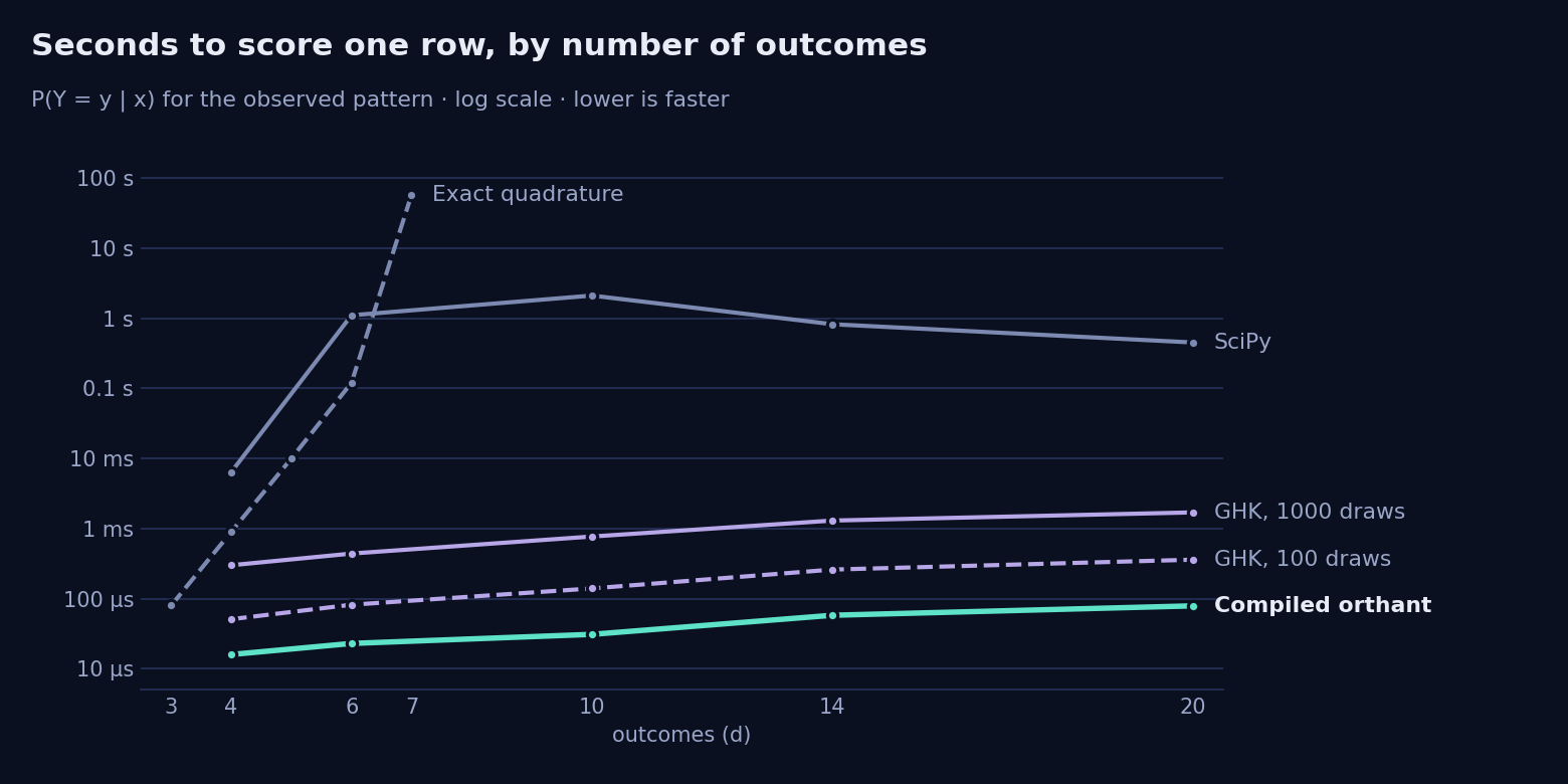
There are three ways to score, and the choice is yours:

The compiled backend ships with the package for Linux on CPython 3.11 and 3.12. Without a key it handles up to three outcomes; a key unlocks the rest. The hosted service is for test sets too large for one machine and comes with the quantecarlo client.

Where it falls short

• It isn't the accuracy leader on every benchmark. On standard multi-label datasets with six labels, ensembles of classifier chains predicted the exact label set more often. The multivariate probit's case is a coherent joint model with readable dependence, not a leaderboard. Benchmark.
• No standard errors yet. Σ is a point estimate.
• Explainable only as far as the parts are. Linear margins give per-outcome coefficients plus Σ, an interpretable model end to end. With XGBoost or random-forest margins, Σ is still readable, but each margin is as much a black box as its classifier.
• Read a correlation as a floor. Prediction error in the per-outcome models pulls the estimated correlations toward zero.
• Binary outcomes only, fully observed.

The full list: limitations.md.